
Process |
Home |
I only started astrophotography in late 2020, but I can say I really *like* this hobby. Yes, some of it is because of its still freshness to me. But a lot of it is because it is not easy. It takes a non-trivial combination of knowledge, patience, intellectual curiosity, and financial resources to pull it off. Yes, this may sound elitist, and it probably is, but that doesn't make it false: few people relatively speaking are capable of taking decent pictures of these objects in deep space thousands of light years away from us.
In this page, I am going to overview my process. This starts with my image capture, then image pre-processing, and finally with image post-processing. I don't have any one particular reason for writing this down. One reason is that I tend to figure out whether I understand something by writing it down. Another is that finding other people's notes was tremendously helpful to me when I was starting, so maybe some other newbie might find this useful. And yet another reason is that this hobby is filled with lots of time when one cannot be imaging due to weather or other reasons, and this is a better time filler than TV.
Reasons aside, this is how I personally go about getting the astrophotos you might have seen posted. At this point, I am more than a year into this hobby so my workflow has grown reasonably complex. If you are just starting astrophotography yourself, you might also want to take a look at my newbie workflow.
My astrophotography process starts with following main stages to get to a "starting" image:
This starting image is what is called a stacked image. To a quick view, it just looks black, but all the detail is actually in there and just needs to be "pulled out" though image processing. I use PixInsight for my image processing, and my current workflow for post-processing comprises the following main steps:
Everyone who does astrophotography has some personal workflow. If you look at an experienced imager, their flow will likely have a few additional processes. However, this set is reasonably complete and the better imagers are just (much) better at using them effectively!
That is the overview of the entire process. In the remaining sections, I will add more details about the individual steps of the process.
For image capture, I use the NINA software package. This extraordinary free (opensource) software controls all aspects of the capture process including camera and mount control, image location and centering, sequencing, creation of all calibration frames, and much more. The imaging pane of NINA is shown below.
These are the important characteristics for my image capture:
My procedure for getting capture up and going is pretty mechanical at this point. Since I now have my setup in a permanent position in my back yard, I don't have any physical setup or polar alignment. It takes maybe 15 minutes from the time I take the Telegizmo cover off to when I can actually start imaging.
And that's it. The sequence will unpark the mount, and cool the camera. Then when the target rises above my custom horizon, it will slew the scope to the target, platesolve and perfectly center it, run autofocus, start guiding, and start taking images. Periodically during imaging, it will check centering and adjust if necessary. It will also dither every 10 minutes, and refocus if the temperature changes by more than 1°C. If a meridian flip is needed, it will do that. Finally, when the target drops below my horizon, it parks the scope and warms the camera. And everything is all parked and ready to be covered when I wake up in the morning!
Before discussing how I take darks, flats, and bias frames, I want to briefly discuss what these are and why we use them. There are any number of excellent tutorials on this that one can find on the web, and the regulars on any of the astronomy forums such as cloudynights will be happy to explain the details. If you are actually starting to *do* astrophotography, I encourage to make use of additional resources on this topic. My purpose here is just an overview for context.
Most people who use digital cameras use them for taking daylight photography. The pictures from even the cheapest digital cameras today produce spectacular images, but one can easily see the limitations of the digital sensor when one takes a picture in a dimly lit area (without flash). The picture is noisy and has bad contrast among other issues. Astrophotography exacerbates these problems to the extreme. The target being imaged is very faint, often only slightly brighter than the background. In constrast to daylight photos, special care and techniques must be applied to produce anything resembling a recognizable image.
There are a couple characteristics of digital sensors that become meaningful in this domain. The first is the notion of "dark current." When a sensor is recording, it will "record" photons due to electrical activity even without any photons present. This read noise varies with the exposure duration and the temperature of the sensor and typically doubles with every 5° Celsius. Note that this is not a constant value but rather varies across the pixels of the sensor. When we take an actual image (called a "light"), we want to remove the effect of this dark current to end up with an image that represent only the photons that arrived from the target.
Here is an example of the dark current that accumulated in a 120s exposure at 16° C. This image has been stretched to more clearly show the effect.

Fortunately, while this dark current depends on exposure time and the sensor temperature, these are all it depends on. Consequently, we can take so called "dark" frames at the same exposure time and temperature as our light frames and use these to correct the lights by subtracting the pixels of this dark frame from the equivalent light frames.
Another characteristic of digital imaging that can be problematic is reading out very small amount of signal. To ensure that we don't get negative values, the sensor electronics will add a small positive "bias" signal. This bias value does not represent actual signal so we want to exclude it. Unfortunately, it is not a single constant value that can be globally subtracted but varies from pixel to pixel. Fortunately, for a particular pixel, it is roughly constant across images so we can measure it once by taking a very fast (so dark current doesn't build up) dark image (with a lens cap on). These frames are called "bias" frames.
The last nuance has more to do with the complete optical train rather than the digital sensor alone. Various effects can cause unevenness of light intensity hitting the sensor. For example, a dust mote on the sensor would cause the area on the mote to be slightly darker, even with the same light intensity hitting the entire sensor. This would show up as a darker spot on your final image. Another effect is the dropoff of light radially from the center of the telescope lens to the edges. This causes a vignetting effect of the final image. Below is an example of the vignetting effect. Note that darker circular areas towards edges of the frame.

Similar to dark current and bias, the vignetting characteristics of the optical train remain the same provided that the optical train has not been modified in any way (for example, to change a filter). Even the dust motes will stay if the setup is undisturbed. Given this, there is an equivalent way of adjusting for the light intensity unevenness. Suppose for example that in our light frame one pixel gets the full intensity of light and some other pixel away from it is only receiving 70% of the light due to either vignetting or a dust mote. If we also take a so called "flat" frame which is just a picture of a plain white image using the same optical train, then the light on equivalent pixels on the flat frame will also be 100% and 70%. Now, if you take the light frame pixels and divide them by the equivalent flat frame pixels, voila! The light frame pixels are corrected to the values they would have without the uneven illumination.
Now with the reason for darks, flats, and bias out of the way, how do we take them. First, for each of these, we do not take a single instance but rather a set of them. We have already covered how I use NINA to take my lights. Recall that darks are at the same exposure time and temperature as the lights, but without any light hitting the sensor. Consequently, it is easy to use the same process as for my lights: cover the telescope opening and take the darks as if they were lights using the same exposure time. (Since I have a cooled astrocam, I can exactly match the sensor temperature.) The bias are simply very fast exposures without light hitting the sensor. This is just like taking a dark (with the scope opening covered) but with exposure time set to a very low value (0.00025s in my case).
The flats are quite a bit different. Proper flats require that evenly diffuse light is captured at an exposure time that puts the histogram somewhere in the middle of the scale. The first problem is the light source used. There are different methods including using natural sky light to using some sort of "light box". I personally use a LED tracing pad ($25 on Amazon) with a few sheets of white paper in front of it (to diffuse the light sufficiently) attached to a foam cutout that allows it to stably sit on top my scope. My contraption is shown below:

The other difficulty in taking flats is getting the exposure time right. NINA actually has a Flats Wizard which supposedly helps with this. So far, I have not quite gotten this to work and instead do it manually. I know that depending on the filter I am using, with my light box it takes either 0.1s or 1s to get the correct exposure. So I take a sanity sample to verify, then I take about 40 exposures using that setting.
The procedure I previously described using flat frames isn't quite correct. Recall that every image has included in it the bias offset on every pixel. And for anything other than very short frames, it also includes dark current. So the light frame values actually contain the light photon counts plus the dark current plus the bias. And the flat frames actually contain the white light plus the bias (because these are very short, the dark current is negligible). Working out the math will show that straight division as implied in the previous paragraph does not give the desired result. It is *close*... but in dealing with images like this that are SO faint relative to the background, even small errors like this make it problematic to get a decent image.
To reiterate, if S is actual interesting signal, D is the dark current, B is the bias, and W is the white light used for the flats, then
Light frame L = S + d + b
Dark frame D = 0 + d + b
Flat frame F = w + 0 + b
Bias frame B = 0 + 0 + b
Now, given a light frame, we can correct for dark current, bias, and uneven light intensity with the following equation:
(L - D) / (F - B) =
[(S + d + b) - (0 + d + b)] / [(w + 0 + b) - (0 + 0 + b)] =
S / w
where S and w have the same attenuation for each pixel.
The above procedure must be done on each light frame. Furthermore, since there is always variation in images read, both for "real" light frames as well as dark, flat, and bias frames, this process actually first combines multiple dark frames into a dark "master", multiple flats into a flat master, and multiple bias frames into a bias master. It is these masters that are used in the equation above on each light frame.
The processing is mechanical but tedious and it has to be handled by software that can do this en mass. I use the PixInsight Weighted-Batch-PreProcessing (WBPP) script for my calibration. The main screen of the 2.1.2 version of the script is shown below.

Along the bottom left, there are tabs for bias, darks, flats, and lights. You select each of these and then add the files in each category. Next, in lower right, set the output directory. Virtually all of my settings are the defaults values, with some of the more important settings below:
There are some additional configurables associated with registration. I will cover these in the Registration section next.
In the next section, I will discuss the Integration process which takes multiple individual images and combines them into a better single image. I will leave the discussion about why we do this to that section but suffice it for now to say that this is a "vertical" combination where the "same" images are stacked on top of each other for the combination. In order for this to work, clearly the pictures have to be aligned exactly the same: if one frame is offset relative to the others, then it will preclude this stacking.
Registration is the process of aligning a sequence of images to some reference image. First, this reference image is selected and some set of stars in the image are identified. Then, for each non-reference image, the same set of stars are identified, and the frame is offset and/or rotated so that the stars in this image exactly align with the stars in reference image. Obviously it is more complicated than this and there are a variety of options in terms of thresholds that determine the stars, the method of doing the alignment, what to do with non-overlapping portions of the frames, etc. However, this general description should give a good enough feel for what happens in this process.
One might ask why the frames need to be aligned in the first place. After all, if you have a tracking mount, doesn't that keep the telescope pointing at exactly the same spot so all the individual frames are automatically aligned by default? Conceptually this is correct but it is a matter of accuracy. Take my setup, for example, which is reasonably typical. My "image scale" is 1.61 arcsec/px. This means that if the telescope pointing is more than 1.61 arcsec off from the last frame, then the photons from each point will end up on the wrong pixel. Well, how much is 1.61 arcsec? There are 60 arcsecs in 1 arc-minute, and 60 arc-minutes in 1 degree. Most people think of a degree as being relatively tiny, but here we are saying that if my mount is off by 0.0004°, the images don't line up. That is simply not possible with non-professional grade mechanics. You have to accept that separate frames will not be exactly aligned and, hence, some type of registration to align them will be necessary.
I also do my registration as part of the PixInsight WBPP processing. The WBPP screen for the registration is shown below.

To include registration in the sequence, I use the following settings:
At the end of the WBPP run, PixInsight puts all the calibrated, debayered, and registered images in a directory. There will be one file for each input light frame. These registered frames are now ready to be stacked as described in the next section.
Integration is the combination of many light frames (calibrated and registered) into a single, higher-quality image. There are two points hinted at in this description. First, it is the combination of many light frames. Second, the combination produces a higher-quality image. Before describing my methodology for integration, let me discuss these two points about integration.
First, why would one use multiple frames? It should be reasonably obvious that Deep Space Objects (DSOs) are very very faint so we need to capture a lot of photons to see anything. One way to get a lot of photons is to take extremely long exposure images. There is a limit to this, however. Remember that to keep a telescope pointed at the exact same spot in the sky, the mount has to exactly track the earth's rotation. As the length of the exposure goes up, the chances that the mount will have enough error to "blur" the image goes up. With the class of mount that I have, for example, even with additional guiding I end up with elongated stars (a symptom of inexact tracking) above 5 minutes of exposure. This is not nearly enough.
The second part of the description suggests that the combination of the multiple frames into one frame results in a higher-quality image than any of the individual frames. This is not generally obvious because most people think of digital sensors as being a "perfect recorder" of the image. In fact, due both to the physics of light and the limitations of electronics, there is noise in the count for each pixel. Suppose that the "true" count for a pixel for the 5 minutes is 100. Due to noise, one interval may record 97, another 101, another 103, etc. The individual frame values are all "wrong". However, an average over a large number of frames starts getting close to the correct value.
The effect of averaging a large number of light frames over a single frame is quite dramatic. Below are examples of a single 180s frame compared to a stack of 100 of these frames. Both have been stretched to show the effect more clearly.


I use the PixInsight Integration process to stack my light frames. The screen for that process is shown below. The primary configurables (other than the listing of the frames to integrate of course) are the method for combining and the method for detecting and removing outliers. For the former, I use averaging. For the latter, I use Windsorized sigma clipping which replaces outliers for a pixel with the median.

At the end of this, we have a "stacked" image. In general, this just looks black because most of the pixel values are very close to the black point. However, the image is really "in there" and can be seen with a temporary contrast "stretch". Note that this is only for viewing: it doesn't actually change the values of the pixels. With the PixInsight software I use, you can see when this temporary stretch is applied by the green highlight in the tab along the left hand side of the image.
Below is the initial stacked image in "linear" form, first as is and then with a temporary stretch. The first set of operations in post-processing work in this "linear" form.


Stacking introduces artifacts around the edges of the image as the individual light frames were shifted and/or rotated during registration. The first step is to crop out the edges.
The dynamic crop process settings I use and the resulting crop region is shown in the following diagram.

The background of the image is generally not even. This can happen for a lot of reasons but in my case it is mostly due to the extreme light pollution (LP). Since this LP is coming from the "ground," one side of the image will be brighter than the other. Note that because the camera is rotating at varying angles relative to the ground depending on where the telescope is pointing, this bright side is not fixed and not necessarily from the bottom: it can be from any side and angle (but generally not from the top down).
The background extraction process is intended to remove these gradients and to produce a more even, neutral background. PixInsight has two such processes but the one I use more often is called the Dynamic Background Extraction (DBE). In this tool, you place samples on the image at points that are supposed to be pure background (i.e. no nebulosity or any part of your target). The following diagram shows the tool settings and the sample points I chose for this particular image.

The tool then builds a background model using a splines fit to those points and then subtracts out that background model. This gives a resulting image with a more even background. Below is the background model created for this image, and then the resulting image with the background model applied.


The "color" captured by the camera isn't generally reasonable "as is" for astro photographs. There are several reasons for this. One is that the standard color matrix used on one-shot-color (OSC) cameras is the Bayer matrix which is RGGB in my case. In other words, there are two green pixels for every one blue and one red. As such, the image will be greener than expected. (The reason it is done this way is that our eyes are more sensitive to green than either red or blue, so having more green pixels produces terrestrial photos with less apparent noise.) Another is that our digital sensors either intentionally filter out or are inherently less sensitive to some wavelengths of light from astronomical objects. Finally, the imaging train itself may include filters that attempt to mitigate light pollution or enhance contrast for emission nebulae.
Regardless of the reason, we are left with an image that is a poor color match. The color calibration step attempts to correct the color. PixInsight has a couple of tools for this but I generally use the newer Photometric Color Calibration. The concept behind this is genius (to me at least). Essentially, you tell the tool what target is in the image and it uses that information to obtain the true color information of the stars around the target from an astronomy database. It then extracts the stars in your image and compares it against the matching stars from the database. Using this, it determines the appropriate color correction to correct your stars to the reference colors. It then applies this correction to the entire image producing an image which is much closer to the "proper" color.
The following diagrams show the tool screen with some of my settings, and the result after applying the tool to the image.


As earth bound observers, we are peering at space objects through the earth's atmosphere. The atmosphere has the characteristics of a fluid and it bends and twists the light rays in unpredictable ways. However, there is a known reference. The image has stars and we know that these are point sources of light. By comparing the actual image of the stars versus what they should look like, one can recreate the "point spread function" that represents how the light was malformed on its way through the atmosphere. Using the point spread function and the Richardson-Lucy algorithm, one can then "undo" some of the effects of the atmosphere. It is more complicated than I explained here and it is not perfect, but this step recovers some of the detail lost to the smearing by the atmosphere.
The first preparatory step for deconvolution is representing the point spread function. This generally involves picking a set of stars that meet certain characteristics (bright enough, not too bright, etc.) and determining a best fit Moffat function to those stars. As one can imagine, this can be tedious and I instead use the excellent PsfImage script by Hartmut Bornemann. The determined PSF is shown in the following diagram.

The Richardson-Lucy algorithm can sometimes (always for me) introduce "ringing" artifacts around bright stars. These are dark rings around the circumference of the star. To avoid these, one can "protect" these bright stars by masking the image with a star mask. The deconvolution algorithm is then effectively applied to the whole image except for the bright stars. Shown below are the star mask settings I use to generate this "dering" mask and the result. We want most of the stars to be deconvolved so this is configured to only capture the largest and brightest stars.


With these preparatory steps complete, the actual deconvolution can be run. Shown below are the settings I typically start with. Note the use of the external PSF function and Local Support. I will usually play with the Iterations and the Global Dark settings until I achieve the desired result.

The before and after outcome of deconvolution is shown below. In general, the stars are tighter and, especially for the smaller ones, brighter. It might be harder to see but the target has additional detail. Note that the background noise is also sharpened but this undesirable aspect is fixed in a subsequent step.


Image post-processing usually involves noise reduction at several points in the process. Right after deconvolution is the first spot at which I apply noise reduction. This is by no means universal, and you will typically see many more variants of noise reduction by experienced imagers.
My tool of choice for noise reduction in the linear phase is the Multiscale Linear Transform. This tool first separates the features of the image into different "scales" (using a mathematical application of wavelets). It then applies different levels of "blurring" at the different scales. This allows it to, for example, clean up the high frequency pixel-to-pixel noise without also blurring the larger size structures that are part of the actual target.
You might have noticed that I talked about deconvolution in the prior step as sharpening the image, and now about noise reduction as blurring. These two produce opposite effects and I do not want to undo the effects of deconvolution with noise reduction. Consequently, I first create a luminance mask which essentially maps the intensity at a pixel to a mask value: bright pixels have a large value and vice versa. This results in the "background" of the image having low mask values and the desired target having high mask values. This mask can then be applied to the image before noise reduction so that the noise reduction effectively mostly affects the background. The diagrams below show the luminance mask I created and the mask applied to the image. The regions in red are "protected" from the noise reduction to be applied.


The MLT noise reduction is then applied to the masked image. These are the settings I typically use for this.

Below is the before and after effect of the MLT noise reduction. As can be seen, the results can be quite dramatic. I will note that many beginner imagers "over do" the noise reduction. The goal here is noise *reduction* not noise removal. If this is too heavy handed, the result is a "plastic" looking image.


All the previous steps were done in the "linear" phase which, as previously described, means that the pixel values are as recorded by the camera (or more correctly, recorded by the camera and then averaged through integration). We see the details in my examples above only because a temporary stretch was applied within PixInsight. However, if we export that image to a JPEG and then use a regular photo viewer to look at it, it will be black. At this point, we "stretch" the image. This is not for viewing only but rather actually modifies the pixel values and creates a new image. This image, when viewed by an external photo application, will show the target in a manner similar to the temporary stretching.
As with all things PixInsight, there are multiple ways of doing stretching. Experienced imagers have their own favorite methods and combinations, sometimes dependent on the specific target. Over the months, I have gravitated to the Masked Stretch as my primary stretching technique. This is a built in process that I have found does a great job at keeping the stars in check and works well as my initial stretch.
The pictures below show my settings for the masked stretch and the outcome. Note that there is no green highlight on the left tab of the result indicating that no temporary stretch is applied, so this is what the image actually looks like now.


One of the more recent changes in my workflow is the incorporation of the StarNet++ tool. This tool, somewhat magically, separates out the stars from an astro image. The advantage of this is that one can then process the image with the target of interest separately from the stars. Different processes can be used to accentuate features in the target only, or deaccentuate in the stars, etc. Then at the end, the two images can be recombined.
If you noticed my use of masks earlier, you might wonder why the same thing could not be effected using masks. Indeed, some imagers do indeed use the masking approach. In general, these tend to be the more experienced imagers as it is considerably more difficult. But StarNet introduces artifacts into the image and the top end imagers find this degradation unacceptable.
The image below shows my settings for the StarNet application.

The outcome of the StarNet application shown below. Clearly there are some remnants of the stars left in the starless image but, all in all, it is quite amazing that this works at all. The capabilities of neural networks seems almost boundless these days.


The Masked Stretch does a great job at an initial stretch but it usually isn't stretched to the final extent that I prefer. Consequently, I will usually add some extra stretching to the target image after having removed the stars. In most cases, I will use the Histogram Transfer Function (HTF), though I have used the Arcsinh stretch on others.
The HTF stretch function in PixInsight has a preview function that shows the potential outcome allowing for very interactive fine tuning. The following image shows the additional stretch curve that I eventually chose for this target.

The following pictures show the image before and after the additional HTF stretch. The effect is subtle but is an improvement.

After stretching, it is common to do some additional noise reduction. Many experienced imagers use TGV Denoise at this stage and I have simply copied that. At this point, we want to limit the noise reduction to the background; if it were applied globally, it would cause the loss of detail on the target parts of the image. To achieve this, one creates a mask and then applies it to the image. For this case, I use a luminosity mask (i.e a mask created based on the luminous portions of the image) and then apply it to protect everything other than the background.
The generated luminosity mask, and the mask applied to the image along with my TGV Denoise settings is shown below. The red areas indicate the regions protected from the TGV Denoise process.


Now the TGVDenoise is applied. The before and after images are shown below. Again, the change is subtle, in keeping with making this noise reduction instead of noise elimination.


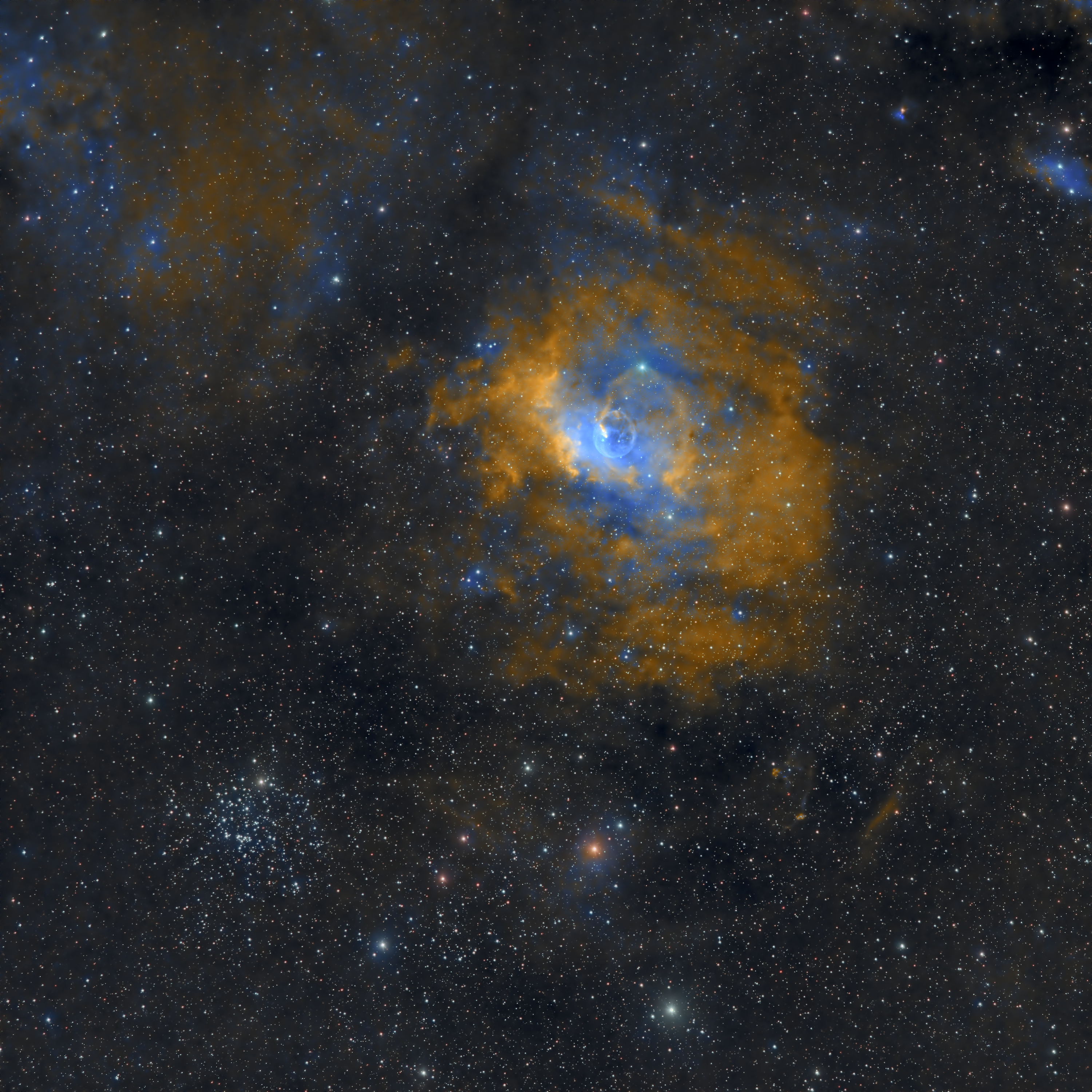
My setup is an OSC setup which is standard RGB palette. Some targets, specifically emission nebula, are essentially all red in this palette. When imaging is done with a dualband filter on emission nebula (I have the L-Enhance dualband filter), one often wants to convert into the "HOO" palette which is a subset of the eponymous Hubble SHO palette. In this palette, the colors represent the three main types of gases in nebula: Ha (hydrogen alpha), OIII (oxygen), and Si (sulfur). While there is scientific merit to this, for us imagers the primary reason is that it produces a more appealing picture than an all-red image.
The Bubble nebula used in this example is an emission nebula captured using the L-Enhance filter, so I chose to convert the palette. With a dualband filter, the Ha wavelength is captured as red and the OIII wavelength as both blue and green. The first step in this process is to split the channels into separate RGB channels. For OSC dualband images, since OIII is captured by both the green and blue channels, and the green channel is stronger (due to the RGGB matrix), most imagers discard the blue channel and use the red channel as Ha and the green channel as OIII. The resulting Ha and OIII from this split is shown in the following.


The next step is then "equalizing" the Ha and OIII images. The Ha output is typically much stronger than OIII so it is generally a process of further stretching the OIII to get the image statistics to more closely match the Ha statistics. The techniques are quite varied here, and this part of it is far more art than science. I won't try to describe this step in more detail as I personally don't have a fixed process here and it's still trial-and-error for me at this stage.
After this step, we have two channels. To map onto our RGB space, we typically map Ha onto Red, and OIII onto Blue. To complete the mapping, we need a channel to map onto Green. If the same OIII is used for Green, then it becomes the true HOO palette. I generally prefer a pseudo HSO where I create Si as a combination of the Ha + OIII. (You will sometimes see this palette written as the H(H+O)O palette.) The weighting used differs but a value of 0.65 Ha + 0.35 OIII is common and is the one I use.
The following shows the pixel math expression I use to create my pseudo-Si and the result.


With the three "color" channels, along with an extracted luminance, I am now ready to combine into a color image in the H(H+O)O palette. I use the PixInsight LRGB combination process with Ha → red, OIII → blue, and pseudo-Si → green.
The images below show my LRGB combination settings and the result.


The previous section was optional and only applied to emission nebula targets. The saturation discussed in this step (and the subsequent steps) generally apply for all my imaging.
By this point, the image now has the contrast needed and a reasonably clean background. However the colors will still look "dull," even more so after stretching as that desaturates it. We need to saturate the colors to make the image bright. In most cases, I am not changing the color (hue), just saturating it. Saturation is done using a curves tool which users of most image processing tools would recognize.
We want to limit the saturation to the target itself. The technique previously described of using a luminance mask to only expose the areas targeted applies here. Below shows the saturation curve I used along with the resulting image. This step makes the colors "pop" but one has to resist the temptation to over-do it.


Sometimes there are areas of the target that could benefit from some additional enhancement of the contrast. In this example, this is not really the case and I wouldn't typically use this step. However, for the sake of showing my process, I will include the steps I use here.
First, we only want to enhance the contrast within a region of interest. Consequently, it needs to be restricted precisely to the area in question. Since these areas are often irregular, I use the fantastic GAME script by Harmut Bornemann. Shown below is the multipoint mask drawn around the area that I want to enhance. Once this is done, the GAME script creates the image mask.

With the mask applied, the localized contrast enhancement can be performed on the area of interest. For this, I use the Local Histogram Equalization tool. This technique of histogram equalization is a general stretching technique but LHE is a specific version applicable to enhancing a portion of an image rather than general stretching.
The LHE settings and the after effect is shown below. Again, the effect is subtle. (This is the case with most of astrophotography post-processing. The individual steps show relatively minor effect, but they add up to a big overall improvement.)


A typical next step is some additional sharpening of the detail in specific areas of the image. There are multiple sharpening tools available in PixInsight, the most commonly used ones being the Multiscale Linear Transform (MLT) and the UnsharpMask (which paradoxically is a sharpening feature). The correct tool depends on what one is trying to sharpen or emphasize. In this example I wanted to sharpen the lower edge of the Bubble so I used the Unsharp Mask.
As with local histogram equalization, sharpening has the side effect of exacerbating any noise that is present. Consequently, it needs to be precisely restricted to the area that requires sharpening. I again used the GAME script to create the mask to expose only the area I wanted to target. The Unsharp Mask settings and the after effect is shown below. This is a somewhat contrived example and I wouldn't normally sharpen here. But hopefully you can see the subtle change along the lower left edge of the Bubble.


With the processing of the actual target complete, I now turn back to the stars which were extracted using the StarNet tool. Some imagers simply add the stars back to the image at this point. For most targets though, I think the stars overwhelm the image and detract from the picture. These are works of art, not scientific images. While I would never add something that wasn't there, I do subscribe to the technique of star reduction as a way of emphasizing my real target.
The basic process in PixInsight for star reduction is the Erosion function of the Morphologial Transform process. I personally don't like the effect of directly applying Erosion to the stars image. This eliminates the smaller stars and dulls all the remaining stars, but it creates a "webbed" look to the image. I have instead settled on a technique derived from Adam Block's method and another method from thecoldestnights.com.
The first step is creating a mask that covers the cores of the medium and larger stars. The method used here is a curves applied to the luminance from the stars image. Below is shown the curve I used to create the star mask, and then the erosion settings to be applied to the masked stars.


Applying the erosion produces a star image with the smaller stars eliminated and the remaining stars shrunk. However, the cores of the remaining stars are at their full intensity, the look that I prefer. Below is a zoomed image showing the difference between the original stars and the reduced stars.


With a completed starless target image and reduced stars image, the next step in my process is the combination of the two into a final image. This is a simple PixelMath operation. The settings I use and the final version of my image is shown below.


That represents my current image collection and processing workflow. At this stage, the image is stored in the PixInsight native format (xisf); I also export as JPG in both full jpeg resolution and downscaled for web viewing. You can see the final version of the image used in this example at this link.
I hope this gives you a good feel for the overall astrophotography process. It might seem daunting, and it is at first, but eventually the steps become routine. I will reiterate that though I am not a rote beginner, I wouldn't consider myself an experienced imager. If you were reading this as a reference, you absolutely should also find and reference the workflow examples from the many experienced individuals on the CloudyNights forum and on YouTube.
Thanks for reading and Cheers!!